2.3. The Gaussian Distribution

• The Gaussian, also known as the normal distribution, is a widely used model for the distribution of continuous variables. For single variable $x$, the Gaussian distribution can be written in the form:

  $$\mathcal{N}(x|\mu,\sigma^2)=\frac{1}{(2\pi\sigma^2)^{1/2}}\exp{\{-\frac{1}{2\sigma^2}(x-\mu)^2\}}\tag1$$

  where $\mu,\sigma^2$ are the mean and the variance respectively.

  

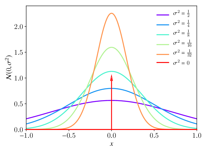
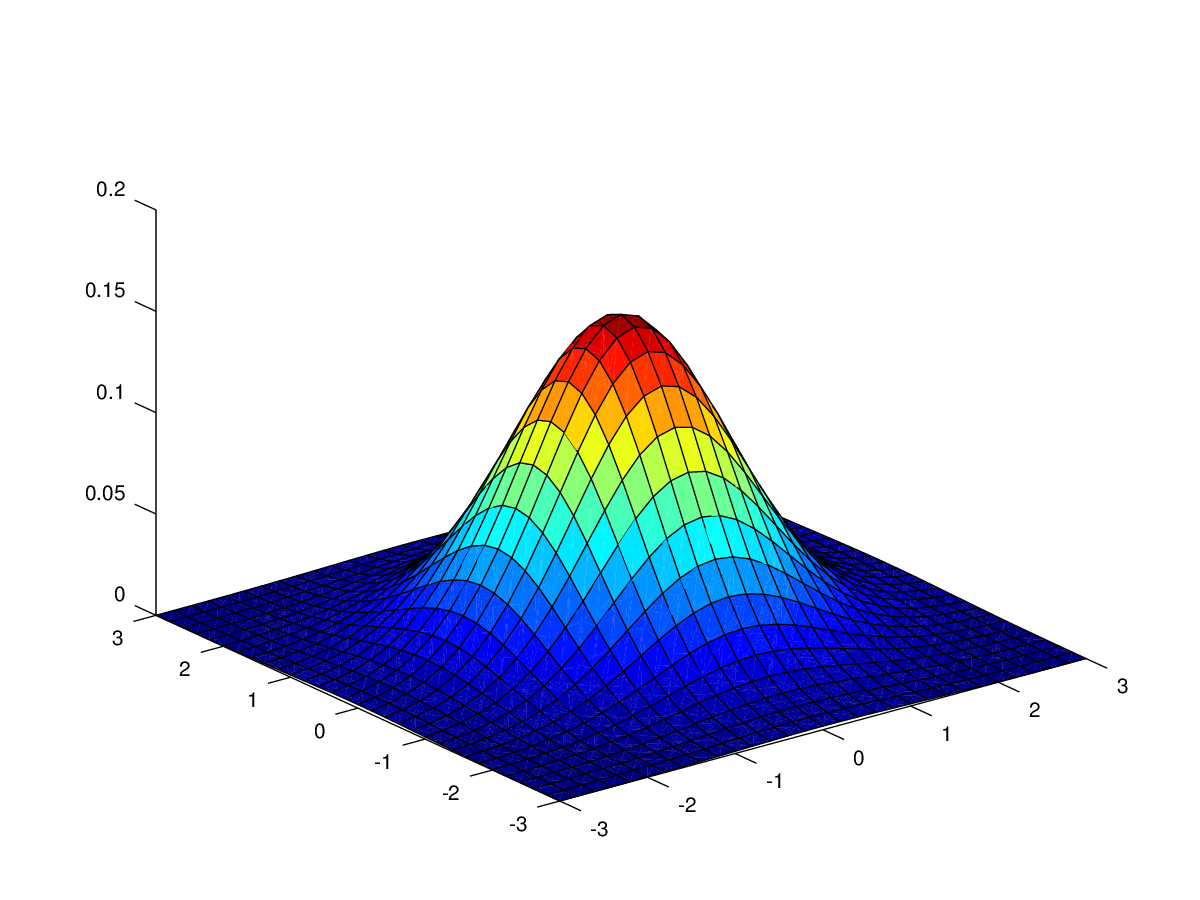
  Figure 1: 1-dimensional Gaussian distribution Source: https://www.researchgate.net/figure/Gaussian-bell-function-normal-distribution-N-0-s-2-with-varying-variance-s-2-For_fig1_334535945

   

• For $D-$dimensional vector $\mathbf{x}$, the multivariate Gaussian distribution takes the form:

  $$\mathcal{N}(\mathbf{x}|\vec\mu,\Sigma)=\frac{1}{(2\pi)^{D/2}|\Sigma|^{1/2}}\exp{\{-\frac{1}{2}(\mathbf{x}-\vec\mu)^\top\Sigma^{-1}(\mathbf{x}-\vec\mu)\}}\tag2$$

  where the mean and the covariance matrix was mentioned in ML&PR_2.

• The Gaussian distribution arises in many different context. For example, Figure 3 plots the mean of $N$ uniformly distributed numbers for various values of $N$:

  

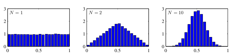
  Figure 3 Source: Pattern Recognition and Machine Learning | C.M.Bishop

• Let consider the geometrical form of the Gaussian distribution:

  $$\Delta^2=(\mathbf{x-\vec\mu})^\top\Sigma^{-1}(\mathbf{x-\vec\mu})\tag3$$

  The $\Delta$ called Mahalanobis distance from $\mathbf{x}$ to $\vec\mu$. In Euclidean distance, $\Sigma$ is identity matrix.

• We know that $\Sigma$ is a symmetric matrix. So, it has only real eigenvalues, specifically $D$ eigenvalues $\lambda_1,...\lambda_D$:

  $$\Sigma\mathbf{u}_i=\lambda_i\mathbf{u}_i\tag4$$

  where $\mathbf{u}_i$ is a eigenvector corresponding to $\lambda_i$. The eigenvectors are chosen to form an orthogonal set such that:

  $$\mathbf{u}_i^\top\mathbf{u}_j=\begin{cases}1 \ \ \ \text{if} \ i=j \\ 0 \ \ \ \text{otherwise}\end{cases}\tag5$$

• We can rewrite $\Sigma$ in the form:

  $$\Sigma=\sum_{i=1}^D\lambda_i\mathbf{u}_i\mathbf{u}_i^\top\tag6$$

  Similarity, we have:

  $$\Sigma^{-1}=\sum_{i=1}^D\frac{1}{\lambda_i}\mathbf{u}_i\mathbf{u}_i^\top\tag7$$

• From $(7)$, $(3)$ becomes:

  $$\begin{align} \Delta^2&=\sum_{i=1}^D\frac{1}{\lambda_i}(\mathbf{x-\vec\mu})^\top\mathbf{u}_i\mathbf{u}_i^\top(\mathbf{x-\vec\mu})\tag8\\ &=\sum_{i=1}^D\frac{1}{\lambda_i}[\mathbf{u}_i^\top(\mathbf{x-\vec\mu})]^\top\mathbf{u}_i^\top(\mathbf{x-\vec\mu})\tag9\\ &=\sum_{i=1}^D(\frac{\mathbf{u}_i^\top(\mathbf{x-\vec\mu})}{\lambda_i^{1/2}})^2\tag{10}\\ &=\sum_{i=1}^D(\frac{\mathbf{y}_i}{\lambda_i^{1/2}})^2\tag{11} \end{align}$$

  where $\mathbf{y}_i=\mathbf{u}_i^\top(\mathbf{x}-\vec\mu)$.

  $(9)=(10)$ because $\mathbf{u}_i^\top(\mathbf{x-\vec\mu})\in\mathcal{R}^1$ so $[\mathbf{u}_i^\top(\mathbf{x-\vec\mu})]^\top\mathbf{u}_i^\top(\mathbf{x-\vec\mu})=[\mathbf{u}_i^\top(\mathbf{x-\vec\mu})]^2$.

• Forming $\mathbf{U}=[\mathbf{u}_1 \ ... \ \mathbf{u}_D]^\top$, we obtain:

  $$\mathbf{y}=[\mathbf{y}_1 \ ... \ \mathbf{y}_D]^\top=\mathbf{U}(\mathbf{x}-\vec\mu)\tag{12}$$

  Note that: $\mathbf{U}$ is a orthogonal matrix.

  If all of eigenvalues $\lambda_i$ are positive, these surfaces represent ellipsoids with center $\vec\mu$ and their axes oriented along $\mathbf{u}_i$. We see that $\mathbf{y}_i$ is a vector $\mathbf{x}-\vec\mu$ projected into $\mathbf{u}_i$ coordinate which scaling factor $\lambda_i^{1/2}$.

  

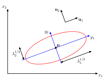
  Figure 4 Source: Pattern Recognition and Machine Learning | C.M.Bishop

• Also, we have:

  $$|\Sigma|=\prod_{i=1}^D\lambda_i\tag{13*}$$

• We now define

  $$\mathbf{J}=\frac{\partial \mathbf{x}}{\mathbf{\partial y}}=\mathbf{U}^\top\tag{14}$$

  Then

  $$|\mathbf{J}|^2=|\mathbf{U^\top}|^2=1\tag{15}$$

• Thus, in the $\mathbf{y}$ coordinate system, the Gaussian distribution takes the form:

  $$p(\mathbf{y})=p(\mathbf{x})|\mathbf{J}|=\prod_{i=1}^D\frac{1}{(2\pi\lambda_i)^{1/2}}\exp{\{-\frac{\mathbf{y}_i^2}{2\lambda_i}\}}\tag{16}$$

  also

  $$\int p(\mathbf{y})d\mathbf{y}=\prod_{i=1}^D\int_{-\infty}^{\infty}\frac{1}{(2\pi\lambda_i)^{1/2}}\exp{\{-\frac{\mathbf{y}_i^2}{2\lambda_i}\}}\text{d}\mathbf{y}_i=1\tag{17}$$

• From $(2)$ we have:

  $$\begin{align} &\frac{1}{(2\pi)^{D/2}|\Sigma|^{1/2}}\int\exp{\{-\frac{1}{2}(\mathbf{x}-\vec\mu)^\top\Sigma^{-1}(\mathbf{x}-\vec\mu)\}}\text{d}\mathbf{x}\\ &=\frac{1}{(2\pi)^{D/2}|\Sigma|^{1/2}}\int\exp{\{-\frac{1}{2}\mathbf{z}^\top\Sigma^{-1}\mathbf{z}\}}\text{d}\mathbf{z}=1\tag{18} \end{align}$$

  where $\mathbf{z=x-\vec\mu}$.

  So:

  $$\begin{align} \mathbb{E}[\mathbf{x}]&=\frac{1}{(2\pi)^{D/2}|\Sigma|^{1/2}}\int\exp{\{-\frac{1}{2}(\mathbf{x}-\vec\mu)^\top\Sigma^{-1}(\mathbf{x}-\vec\mu)\}}\mathbf{x}\text{d}\mathbf{x}\\ &=\frac{1}{(2\pi)^{D/2}|\Sigma|^{1/2}}\int\exp{\{-\frac{1}{2}\mathbf{z}^\top\Sigma^{-1}\mathbf{z}\}}(\mathbf{z+\vec\mu})\text{d}\mathbf{z}\tag{19}\\ &=\frac{1}{(2\pi)^{D/2}|\Sigma|^{1/2}}(\int\exp{\{-\frac{1}{2}\mathbf{z}^\top\Sigma^{-1}\mathbf{z}\}}\mathbf{z}\text{d}\mathbf{z}+\int\exp{\{-\frac{1}{2}\mathbf{z}^\top\Sigma^{-1}\mathbf{z}\}}\vec\mu\text{d}\mathbf{z})\tag{20}\\ &=\frac{1}{(2\pi)^{D/2}|\Sigma|^{1/2}}(\int\mathbb{A}\text{d}\mathbf{z}+\vec\mu\int\mathbb{B}\text{d}\mathbf{z})\tag{21} \end{align}$$

  where $\mathbb{A}=\exp{\{-\frac{1}{2}\mathbf{z}^\top\Sigma^{-1}\mathbf{z}\}}\mathbf{z}$ and $\mathbb{B}=\exp{\{-\frac{1}{2}\mathbf{z}^\top\Sigma^{-1}\mathbf{z}\}}$.

  We see that $\mathbb{A}$ is an odd function, then $\displaystyle\int\mathbb{A}\text{d}\mathbf{z}=0$.

  From $(18)$ and $(21)$, we have $\vec\mu\frac{1}{(2\pi)^{D/2}|\Sigma|^{1/2}}\displaystyle\int\mathbb{B}\text{d}\mathbf{z}=\vec\mu$.

  Therefore,

  $$\mathbb{E}[\mathbf{x}]=\vec\mu\tag{22}$$

• Let consider second order moments of the Gaussian - $\mathbb{E}[\mathbf{xx^\top}]$:

  $$\begin{align} \mathbb{E}[\mathbf{xx^\top}]&=\frac{1}{(2\pi)^{D/2}\Sigma^{1/2}}\int\exp{\{-\frac{1}{2}(\mathbf{x-\vec\mu)}^\top\Sigma^{-1}\mathbf{(x-\vec\mu)}\}\mathbf{xx^\top}\text{d}\mathbf{x}}\tag{23}\\ &=\frac{1}{(2\pi)^{D/2}\Sigma^{1/2}}\int\exp\{-\frac{1}{2}\mathbf{z^\top}\Sigma^{-1}\mathbf{z}\}(\mathbf{z+\vec\mu})(\mathbf{z+\vec\mu})^\top\text{d}\mathbf{z}\tag{24}\\ &=\frac{1}{(2\pi)^{D/2}\Sigma^{1/2}}(\int\exp\{-\frac{1}{2}\mathbf{z^\top}\Sigma^{-1}\mathbf{z}\}\mathbf{zz^\top}\text{d}\mathbf{z}+\int\exp\{-\frac{1}{2}\mathbf{z^\top}\Sigma^{-1}\mathbf{z}\}\mathbf{\vec\mu\vec\mu^\top}\text{d}\mathbf{z})\tag{25} \end{align}$$

  $(24)=(25)$ because $\exp\{-\frac{1}{2}\mathbf{z^\top}\Sigma^{-1}\mathbf{z}\}(\mathbf{z\vec\mu^\top+\vec\mu z^\top})$ is an odd function so the integral is equal zero.

  We now consider:

  $$\begin{align} &\frac{1}{(2\pi)^{D/2}\Sigma^{1/2}}\int\exp\{-\frac{1}{2}\mathbf{z^\top}\Sigma^{-1}\mathbf{z}\}\mathbf{zz^\top}\text{d}\mathbf{z}\\ &=\frac{1}{(2\pi)^{D/2}\Sigma^{1/2}}\sum_{i=1}^D\sum_{j=1}^D\mathbf{u}_i\mathbf{u}_j^\top\int\exp\{-\sum_{k=1}^D\frac{y_k^2}{2\lambda_k}\}y_iy_j\text{d}\mathbf{y}\tag{26}\\ &=\frac{1}{(2\pi)^{D/2}\Sigma^{1/2}}\sum_{i=1}^D\mathbf{u}_i\mathbf{u}_i^\top\int\exp\{-\sum_{k=1}^D\frac{y_k^2}{2\lambda_k}\}y_i^2\text{d}\mathbf{y}\tag{27}\\ &=\frac{1}{(2\pi)^{D/2}\prod_{j=1}^D\lambda_j^{1/2}}\sum_{i=1}^D\mathbf{u}_i\mathbf{u}_i^\top\int\exp\{-\sum_{k=1}^D\frac{y_k^2}{2\lambda_k}\}y_i^2\text{d}\mathbf{y}\tag{28}\\ &=\sum_{i=1}^D\mathbf{u}_i\mathbf{u}_i^\top\int y_i^2\prod_{j=1}^D\frac{1}{(2\pi\lambda_j)^{1/2}}\exp\{-\frac{y_j^2}{2\lambda_j}\}\text{d}y_j\tag{29}\\ &=\sum_{i=1}^D\mathbf{u}_i\mathbf{u}_i^\top(\int\frac{1}{(2\pi\lambda_1)^{1/2}}\exp\{-\frac{y_1^2}{2\lambda_1}\}\text{d}y_1\times...\times \int\frac{1}{(2\pi\lambda_i)^{1/2}}\exp\{-\frac{y_i^2}{2\lambda_i}\}y_i^2\text{d}y_i\times...\times \int\frac{1}{(2\pi\lambda_D)^{1/2}}\exp\{-\frac{y_D^2}{2\lambda_D}\}\text{d}y_D)\tag{30}\\ &=\sum_{i=1}^D\mathbf{u}_i\mathbf{u}_i^\top(1\times...\times\lambda_i\times...\times1)=\sum_{i=1}^D\mathbf{u}_i\mathbf{u}_i^\top\lambda_i=\Sigma\tag{31} \end{align}$$

  • We have $(26)$ because from $(12)$ we obtain:

    $$\mathbf{z}=\mathbf{U}^{-1}\mathbf{y}=\mathbf{U^\top y}=\sum_{i=1}^D\mathbf{u}_iy_i\tag{32}$$

  • $(26)=(27 )$ because $\mathbf{U}$ is an orthogonal matrix so $\mathbf{u}_i\mathbf{u}_j^\top=\mathbf{0} \ \forall i\ne j$.

  • $(27)=(28)$ because of $(13)$.

  • We have $(28)=(29)$ from $(16)(17)$, have $(31)$ from $(6)$.

  • $(29)=(30)$ because from $(1)$ we have

    $$\int\frac{1}{(2\pi\sigma^2)^{1/2}}\exp{\{-\frac{1}{2\sigma^2}(x-\mu)^2\}}\text{d}x=1\tag{33*}$$

  Thus

  $$\mathbb{E}[\mathbf{xx^\top}]=\vec\mu\vec\mu^\top+\Sigma\tag{34}$$

Appendix (*)

1. The product of the eigenvalues is the determinant of a matrix:

   $$|\Sigma|=\prod_i\lambda_i\tag{13*}$$

   Proof:

   • First, we analysis $\Sigma$ to:

     $$\Sigma=\mathbf{P}\text{diag}(\lambda_1,...,\lambda_n)\mathbf{P}^{-1}\tag{35}$$

   • Use the property of determinant $|\mathbf{AB}|=|\mathbf{BA}|$, we have:

     $$\begin{align}<br>|\Sigma|&=|\mathbf{P}\text{diag}(\lambda_1,...,\lambda_n)\mathbf{P}^{-1}|\tag{36}\\<br>&=|\text{diag}(\lambda_1,...,\lambda_n)\mathbf{P}^{-1}\mathbf{P}|\tag{37}\\<br>&=|\text{diag}(\lambda_1,...,\lambda_n)\mathbf{I}|\tag{38}\\<br>&=\prod_i\lambda_i<br>\end{align}$$

2. The integral of Gaussian is 1:

   $$\int\frac{1}{(2\pi\sigma^2)^{1/2}}\exp{\{-\frac{1}{2\sigma^2}(x-\mu)^2\}}\text{d}x=1\tag{33*}$$

   We have to prove

   $$\int\exp\{-\frac{(x-\mu)^2}{2\sigma^2}\}\text{d}x=(2\pi\sigma^2)^{1/2}\tag{39}$$

   Proof:

   $$\begin{align}<br>\int\exp\{-\frac{(x-\mu)^2}{2\sigma^2}\}\text{d}x&=\int\exp\{-\frac{x^2}{2\sigma^2}\}\text{d}x\tag{40}\\<br>&=\int\exp\{-(\frac{x}{\sqrt{2\sigma^2}})^2\}\text{d}x\tag{41}\\<br>&=(2\sigma^2)^{1/2}\int\exp\{-x^2\}\text{d}x\tag{42}<br>\end{align}$$

   • We now prove $\displaystyle\int\exp\{-x^2\}\text{d}x=\pi^{1/2}$. We have:

     $$\begin{align}<br>(\int_{-\infty}^{+\infty}e^{-x^2}\text{d}x)^2&=\int_{-\infty}^{+\infty}e^{-x^2}\text{d}x\int_{-\infty}^{+\infty}e^{-y^2}\text{d}y\tag{43}\\<br>&=\int_{-\infty}^{+\infty}\int_{-\infty}^{+\infty}e^{-(x^2+y^2)}\text{d}x\text{d}y\tag{44}<br>\end{align}$$

     Set $x=r\cos(\theta)$, $y=r\sin(\theta)$, we have:

     $$\begin{align}<br>(43)&=\int_0^{2\pi}\int_0^{+\infty}e^{-r^2}r \ \text{d}r \text{d}\theta\tag{45}\\<br>&=\int_0^{2\pi}\frac{1}{2}\text{d}\theta=\pi\tag{46}<br>\end{align}$$

     So, we have just prove

     $$\displaystyle\int\exp\{-x^2\}\text{d}x=\pi^{1/2}\tag{47}$$

     Then, $(33^*)$ was proved.

Reference:

• 2.3 | Pattern Recognition and Machine Learning | C.M.Bishop.
• Gaussian integrals | University of Michigan.