• We have introduced the matrix decomposition in DL_1 which have many applications. In this article, we will discuss about using the matrix decomposition to obtain the best possible approximation of a given matrix, called a matrix of low rank.
• A low rank approximation can be considered a compression of the data represented by the given matrix.

2.8 The Singular Value Decomposition (SVD)

• We know that a matrix is not square, the eigendecomposition is not define and we must use a SVD instead.

• Recall about the eigendecomposition, we analyze a matrix $\mathbf{A}$ rely on its eigenvalues and eigenvectors:

  $$\mathbf{A}=\mathbf{V}\text{diag}(\vec\lambda)\mathbf{V}^{-1}\tag1$$

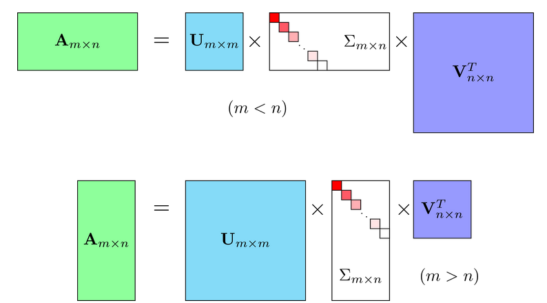
• In SVD, suppose $\mathbf{A}$ is an $m\times n$ matrix, we have:

  $$\mathbf{A}_{m\times n}=\mathbf{U}_{m\times m}\mathbf{D}_{m\times n}\mathbf{V}^\top_{n\times n}\tag2$$

• In there, $\mathbf{D}$ is a diagonal matrix. The element along the diagonal of $\mathbf{D}$, which are $\lambda_1\ge\lambda_2\ge...\ge\lambda_r\ge0=0=...=0$ are known as the singular values of $\mathbf{A}$ and $r$ is rank of $\mathbf{A}$.

2.8.1. The origin of SVD

• From $(2)$, we have:

  $$\begin{align} \mathbf{A}\mathbf{A}^\top&=\mathbf{U}\mathbf{D}\mathbf{V}^\top(\mathbf{U}\mathbf{D}\mathbf{V}^\top)^\top\\ &=\mathbf{U}\mathbf{D}\mathbf{V}^\top\mathbf{V}\mathbf{D^\top}\mathbf{U^\top}\\ &=\mathbf{U}\mathbf{D}\mathbf{D^\top}\mathbf{U^\top} \ \ \ \text{(because $V$ is a orthogonal matrix, so $V^\top V=I$)}\\ &=\mathbf{U}\mathbf{D}\mathbf{D^\top}\mathbf{U}^{-1} \ \ \ \text{($U$ is a orthogonal matrix, so $U^\top=U^{-1}$)}\tag3 \end{align}$$
  • We see that the element in the diagonal of $\mathbf{D}\mathbf{D}^\top$ are $\lambda_1^2, \lambda_2^2,...$ (as we denote in DL_1). Thus, $\lambda_1^2, \lambda_2^2,...$ are the eigenvalues of $\mathbf{A}\mathbf{A}^\top$ and $(3)$ is the eigendecomposition of $\mathbf{A}\mathbf{A}^\top$.
  • Because of $\lambda_i^2\ge0$, $\mathbf{A}\mathbf{A}^\top$ is a positive semidefinite matrix. The values $\lambda_1,...$ are called singular values of $\mathbf{A}$.
  • The columns of matrix $\mathbf{U}$ are eigenvectors of $\mathbf{A}\mathbf{A}^\top$, called left-singular vectors of $\mathbf{A}$.

• Similarity, we can obtain:

  $$\mathbf{A}^\top\mathbf{A}=\mathbf{V}\mathbf{D}\mathbf{D^\top}\mathbf{V}^{-1}\tag4$$

  Therefore, we can show that the columns of matrix $\mathbf{V}$ are the eigenvectors of $\mathbf{A}^\top\mathbf{A}$, called right-singular vectors of $\mathbf{A}$.

  Both $\mathbf{U}$ and $\mathbf{V}$ are orthogonal matrices.

2.8.2. Compact SVD

• We can rewrite $(2)$ to:

  $$\mathbf{A}=\lambda_1\mathbf{u}_1\mathbf{v}_1^\top+\lambda_2\mathbf{u}_2\mathbf{v}_2^\top+...+\lambda_r\mathbf{u}_r\mathbf{v}_r^\top\tag5$$

  where each $\text{rank}(\mathbf{u}_i\mathbf{v}_i^\top)=1$ ($1\le i\le r$).

• We see that $\mathbf{A}$ depends only on the first $r$ columns of $\mathbf{U}$, $\mathbf{V}$ and $r$ values which are nonzero on the diagonal of $\mathbf{D}$. So:

  $$\mathbf{A}=\mathbf{U}_r\mathbf{D}_r(\mathbf{V}_r)^\top\tag6$$

  where $\mathbf{U}_r,\mathbf{V}_r$ included first $r$ columns of $\mathbf{U}$ and $\mathbf{V}_r$, $\mathbf{D}_r$ included first $r$ rows of $\mathbf{D}$.

2.8.3. Truncated SVD

• We already know that the element in the diagonal of $\mathbf{D}$ are nonzero and decrease $\lambda_1\ge\lambda_2\ge...\ge\lambda_r\ge0=0=...=0$. In reality, some value $\lambda_i$ is a big value, the remainder is small, approximately zero. Thus, we can approximate $\mathbf{A}$ by:

  $$\begin{align} \mathbf{A}\approx\mathbf{A}_k&=\mathbf{U}_k\mathbf{D}_k(\mathbf{V}_k)^\top\\ &=\lambda_1\mathbf{u}_1\mathbf{v}_1^\top+\lambda_2\mathbf{u}_2\mathbf{v}_2^\top+...+\lambda_k\mathbf{u}_k\mathbf{v}_k^\top \end{align}\tag7$$

  where $k< r$.

• Theorem:

  $$||\mathbf{A}-\mathbf{A}_k||_F^2=\sum_{i=k+1}^r\lambda_i^2\tag8$$

  It means error of this approximate way is square root of the sum of squares of singular values that we omitted at the end of $\mathbf{D}$.

  • Prove:

    We have $||\mathbf{X}||_F^2=\text{trace}(\mathbf{X}\mathbf{X}^\top)$ and $\text{trace}(\mathbf{X}\mathbf{Y})=\text{trace}(\mathbf{Y}\mathbf{X})$. Now we infer:

    $$\begin{align} ||\mathbf{A}-\mathbf{A}_k||_F^2&=||\sum_{i=k+1}^r\lambda_i\mathbf{u}_i\mathbf{v}_i^\top||_F^2\tag9\\ &=\text{trace}\{(\sum_{i=k+1}^r\lambda_i\mathbf{u}_i\mathbf{v}_i^\top)(\sum_{i=k+1}^r\lambda_i\mathbf{u}_i\mathbf{v}_i^\top)^\top\}\tag{10}\\ &=\text{trace}\{\sum_{i=k+1}^r\sum_{j=k+1}^r\lambda_i\lambda_j\mathbf{u}_i\mathbf{v}_i^\top\mathbf{v}_j\mathbf{u}_j^\top\}\tag{11}\\ &=\text{trace}\{\sum_{i=k+1}^r\lambda_i^2\mathbf{u}_i\mathbf{u}_i^\top\}\tag{12}\\ &=\text{trace}\{\sum_{i=k+1}^r\lambda_i^2\mathbf{u}_i^\top\mathbf{u}_i\}\tag{13}\\ &=\text{trace}\{\sum_{i=k+1}^r\lambda_i^2\}\tag{14}\\ &=\sum_{i=k+1}^r\lambda_i^2\tag{15}\\ \end{align}$$

    $(11)=(12),(13)=(14)$ because $\mathbf{U},\mathbf{V}$ are orthogonal matrices.

    $(12)=(13)$ because of the commutative property of $\text{trace}$ function.

    $(14)=(15)$ because $\sum_{i=k+1}^r\lambda_i^2$ is a scalar.

• Therefore, we obtain:

  $$\frac{||\mathbf{A}-\mathbf{A}_k||_F^2}{||\mathbf{A}||_F^2}=\frac{\sum_{i=k+1}^r\lambda_i^2}{\sum_{i=1}^r\lambda_i^2}\tag{16}$$

  We see that the bigger the $k$ is, the smaller the lost of $\mathbf{A}_k$ (compare to the origin matrix $\mathbf{A}$) is. So we use Truncated SVD to approximate the origin matrix base on the amount of information we want to keep, called Low-rank approximation.

Advance

Prove the existence of SVD:

Theorem: If $\mathbf{A}$ is a real $m\times n$ matrix then there exist orthogonal matrices

such that

where $r=\min(m,n)$ and $\lambda_1\ge...\ge\lambda_r\ge0$. Equivalently:

Proof: Let $\mathbf{x}\in\mathcal{R}^{n},\mathbf{y}\in\mathcal{R}^{m}$ be unit vector. We consider:

• The scalar $z$ must achieve a maximum value on the set $\mathcal{S}=\{\mathbf{x},\mathbf{y}|\mathbf{x}\in\mathcal{R}^{n},\mathbf{y}\in\mathcal{R}^{m},||\mathbf{x}||=||\mathbf{y}||=1\}$. Let $\mathbf{u}_1,\mathbf{v}_1$ be two unit vectors in $\mathcal{R}^m$ and $\mathcal{R}^n$ respectively where this $z$ is achieved maximum $\lambda_1$:

• The maximum value of $z$ is dot product between $\mathbf{u}_1$ and $\mathbf{Av}_1$ then $\mathbf{u}_1$ is parallel to the vector $\mathbf{Av}_1$. Also, we have $\mathbf{u}_1^\top\mathbf{Av}_1=\mathbf{v}_1^\top\mathbf{A^\top u}_1$. Similarity, we can show that $\mathbf{v}_1$ is parallel to the vector $\mathbf{A^\top u}_1$.
• $\mathbf{u}_1,\mathbf{v}_1$ can be extended into orthonormal bases for $\mathcal{R}^m,\mathcal{R^n}$. Collect the orthonormal basis vector from $\mathcal{R}^m,\mathcal{R^n}$ into orthogonal matrices $\mathbf{U}_1,\mathbf{V}_1$ respectively, we have:

• We can show that the first column of $\mathbf{AV}_1$ is $\mathbf{Av}_1=\lambda_1\mathbf{u}_1$ (considered as a exercise for you). So the first entry of $\mathbf{U}_1^\top\mathbf{AV}_1$ is $\mathbf{u}_1^\top\lambda_1\mathbf{u}_1=\lambda_1$ and its other entries are $\mathbf{u}_j^\top\mathbf{A}\mathbf{v}_1=0$ because $\mathbf{Av}_1$ is parallel to $\mathbf{u}_1$ and $\mathbf{u}_1\bot \mathbf{u}_{i(i\ne 1)}$ (because $\mathbf{U_1}$ is orthonormal basis). Thus, we have just explained the result of first column of $\mathbf{S}_1$. Similarity with the first row of $\mathbf{S}_1$, by $\mathbf{u}_1\mathbf{Av}_2=...=\mathbf{u}_1\mathbf{Av}_n=0$. The matrix $\mathbf{A}_1\in\mathcal{R}^{(m-1)\times(n-1)}$. We have:

So:

We repeat until $\mathbf{A}_k$ has zero rows and zeros columns to obtain:

where $\mathbf{U}$ and $\mathbf{V}$ are orthogonal matrices obtained by multiplying together all the orthogonal matrices used in the procedure, and:

Equivalently:

which is the desired result.

• Next, we show that $\lambda_1\ge...\ge\lambda_p$. To show this, we just need to show that $\lambda_2\le\lambda_1$. We have:

  $$\begin{align} \lambda_2&=\max_{||\hat{\mathbf{x}}||=||\hat{\mathbf{y}}||=1}\hat{\mathbf{y}}^\top\mathbf{A}_1\hat{\mathbf{x}}\tag{29}\\ &=\max_{||\hat{\mathbf{x}}||=||\hat{\mathbf{y}}||=1}\begin{bmatrix}0&\hat{\mathbf{y}}\end{bmatrix}^\top\mathbf{S}_1\begin{bmatrix}0\\\hat{\mathbf{x}}\end{bmatrix}\tag{30}\\ &=\max_{||\hat{\mathbf{x}}||=||\hat{\mathbf{y}}||=1}\begin{bmatrix}0&\hat{\mathbf{y}}\end{bmatrix}^\top\mathbf{U}_1^\top\mathbf{AV}_1\begin{bmatrix}0\\\hat{\mathbf{x}}\end{bmatrix}\tag{31}\\ &=\max_{||\hat{\mathbf{x}}||=||\hat{\mathbf{y}}||=1\\\mathbf{x^\top v}_1=\mathbf{y^\top u}_1=0}\mathbf{y^\top Ax}\tag{32} \end{align}$$

  where

  $$\mathbf{x}=\mathbf{V}_1\begin{bmatrix}0\\\hat{\mathbf{x}}\end{bmatrix}\tag{33}$$

  and

  $$\mathbf{y}=\mathbf{U}_1\begin{bmatrix}0\\\hat{\mathbf{y}}\end{bmatrix}\tag{34}$$

  We see that $\mathbf{x}$ is a linear combination of $\mathbf{v}_2,...,\mathbf{v}_n$ and therefore it is unit vector and orthogonal to $\mathbf{v}_1$. Similarity, we can obtain $\mathbf{y}$ is unit vector and $\mathbf{y}\bot\mathbf{u}_1$. So $\mathbf{x,y}$ belong to subsets of the unit spheres in $\mathcal{R^n,R^m}$ respectively. As we assumed above, $\lambda_1=\max z(\mathbf{x,y})$, therefore $\lambda_2\le\lambda_1$.

• Finally, we must prove $\lambda_i$ are nonnegative. We see that $z(\mathbf{x,y})=-z(\mathbf{-x,y})$. Obviously, $\max z(\mathbf{x,y})\ge0$.

   

Reference:

• 2.7 | Deep Learning | Ian Goodfellow, Yoshua Bengio, Aaron Courville.
• Bài 26: Singular Value Decomposition
• 10. Singular Value Decomposition | Duke Computer Science