2.1. Binary variables

• Let imagine when flip a coin, the outcome $x$ is 'heads' or 'tails'. We represent it by numerals $x=1$ representing 'heads' and $x=0$ representing 'tails'. Now we call $x$ is binary variable.

• The probability of $x=1$ will be denoted by the parameter $\mu$ where $0\le\mu\le1$:

  $$p(x=1|\mu)=\mu\tag1$$

  and $p(x=0|\mu)=1-\mu$. The probability distribution of $x$ is a Bernoulli distribution:

  $$\text{Bern}(x|\mu)=\mu^x(1-\mu)^{1-x}\tag2$$

  And we have:

  $$\begin{align} \mathbb{E}[x]&=\mu\tag3\\ \text{var}[x]&=\mu(1-\mu)\tag4 \end{align}$$

• In general, when we flip a coin $N$ times and $x=1$ appears $m$ times. This is called Binomial distribution:

  $$\text{Bin}(m|N,\mu)=\begin{pmatrix}<br>N\\m<br>\end{pmatrix}<br>\mu^m(1-\mu)^{N-m}\tag5$$

  where

  $$\begin{pmatrix} N\\m \end{pmatrix}=\frac{N!}{(N-m)!m!}\tag6$$

  And:

  $$\begin{align} \mathbb{E}[m]&=N\mu\tag7\\ \text{var}[m]&=N\mu(1-\mu)\tag8 \end{align}$$

2.1.1. Beta distribution

• Suppose we have a observed data set $\mathcal{D}=\{x_1,...,x_N\}$. We have to determine $\mu$ so that $p(\mathcal{D}|\mu)$ is the largest. This is Maximum Likelihood method that we will refer later. You just need to know now:

  $$\mu_{ML}=\frac{1}{N}\sum_{i=1}^Nx_i\tag9$$

• If we just have a small data set, for instance $\mathcal{D}=\{1,0,1\}$, if we use formula $(9)$, we have $\mu=0.667$. Intuitively, we know that is not reasonable.

• In order to fix this problem, we could choose a prior to be proportional $\mu$ and $1-\mu$, then the posterior distribution, which is proportional to the product of the prior and likelihood function, will have same functional form as both the prior and likelihood. This property is called conjugacy. We choose a prior, called the Beta distribution:

  $$\text{Beta}(\mu|a,b)=\frac{\Gamma(a+b)}{\Gamma(a)\Gamma(b)}\mu^{a-1}(1-\mu)^{b-1}\tag{10}$$

  where Gamma function has been introduced in MATH_4, just to make sure that:

  $$\int_0^1\text{Beta}(\mu|a,b)\text{d}\mu=1\tag{11}$$

• The mean and variance of the Beta distribution:

  $$\begin{align} \mathbb{E}[\mu]&=\frac{a}{a+b}\tag{12}\\ \text{var}[\mu]&=\frac{ab}{(a+b)^2(a+b+1)}\tag{13} \end{align}$$

• The parameters $a$ and $b$ are called hyperparameters because they control the distribution of the $\mu$.

  

  Figure 1

• The posterior distribution of $\mu$ is now obtained by multiplying the beta prior $(10)$ by the binomial likelihood function $(5)$ and normalizing. Keep only the factors that depends on $\mu$, we have:

  $$p(\mu|m,l,a,b)\propto\mu^{m+a-1}(1-\mu)^{l+b-1}\tag{14}$$

  where $l=N-m$ corresponds the number of 'tails'. Formula $(14)$ could normalize like a other beta distribution:

  $$p(\mu|m,l,a,b)=\frac{\Gamma(m+a+l+b)}{\Gamma(m+a)\Gamma(l+b)}\mu^{m+a-1}(1-\mu)^{l+b-1}\tag{15}$$

  

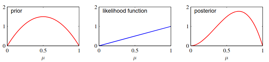
  Figure 2

• If we have a observes data set $\mathcal{D}$, using $(12)$ we obtain:

  $$\mathbb{E}[\mu]=p(x=1|\mathcal{D})=\frac{m+a}{m+a+l+b}\tag{16}$$

  If $l,m\to\infty$, the result $(16)$ is approach to the maximum likelihood result $(9)$.

• In Figure 1, we see that as the number of observations increases, the posterior distribution becomes more sharply, because in formula $(13)$, when $a\to\infty$ or $b\to\infty$, the variance goes to zero. In other word, we observe more and more data, the uncertainty represented by the posterior distribution will decrease. To address this, we take a frequentist view, inference problem for parameter $\theta$ for which we have observed a data set $\mathcal{D}$, described by the joint distribution $p(\theta, \mathcal{D})$:

  $$\mathbb{E}_\theta[\theta]=\mathbb{E}_\mathcal{D}[\mathbb{E}_\theta[\theta|\mathcal{D}]]\tag{17}$$

  where

  $$\begin{align} \mathbb{E}_\theta[\theta]&=\int p(\theta)\theta\text{d}\theta\tag{18}\\ \mathbb{E}_\mathcal{D}[\mathbb{E}_\theta[\theta|\mathcal{D}]]&=\int[\int p(\theta|\mathcal{D})\theta\text{d}\theta\ ] \ p(\mathcal{D})\text{d}\mathcal{D}\tag{19}\\ \end{align}$$

• This result says that the posterior mean of $\theta$, averaged over the distribution generating the data is equal to the prior mean of $\theta$.

• And we can show that:

  $$\mathbb{var}_\theta[\theta]=\mathbb{E}_\mathcal{D}[\mathbb{var}_\theta[\theta|\mathcal{D}]]+\mathbb{var}_\mathcal{D}[\mathbb{E}_\theta[\theta|\mathcal{D}]]$$

Reference:

• 2.1 | Pattern Recognition and Machine Learning | C.M.Bishop.